SQL Structs & Arrays Project
Background
Structs and arrays are powerful container types in SQL that allow us to store complex, hierarchical data within a single column. While they may appear similar, they serve different purposes. Arrays store multiple values of a single data type, such as an array of strings, while structs can hold multiple fields of varying types. This flexibility makes structs ideal for modeling real-world entities with multiple attributes. Their full potential is realized when combined: for example, a column can store an array of structs, and each struct can contain detailed, structured information. This project demonstrates how to use structs and arrays effectively in SQL, particularly within Google BigQuery. The dataset and structure are entirely hypothetical and intended solely for learning and demonstration purposes.
Creating Tables / Inserting Data
The code below creates the tables used in this demonstration and inserts sample data into them.
Creating Tables:
CREATE TABLE test.cruise_passengers (
room_id INT64,
beds INT64,
price_per_night FLOAT64,
passenger STRUCT<
pass_id INT64,
name STRING,
age INT64,
race STRING,
preferences STRUCT<
dining_times ARRAY<STRING>,
food_allergies ARRAY<STRING>,
activity_interests ARRAY<STRING>
>,
onboard_purchases ARRAY<STRUCT<
item STRING,
cost FLOAT64,
purchase_date DATE
>>
>
);
Inserting Data:
INSERT INTO test.cruise_passengers (room_id, beds, price_per_night, passenger) VALUES
(108, 2, 421.00, STRUCT<
pass_id INT64, name STRING, age INT64, race STRING,
preferences STRUCT<dining_times ARRAY<STRING>, food_allergies ARRAY<STRING>, activity_interests ARRAY<STRING>>,
onboard_purchases ARRAY<STRUCT<item STRING, cost FLOAT64, purchase_date DATE>>
>(
1, "Alice", 34, "Asian",
STRUCT(["Breakfast"], CAST([] AS ARRAY<STRING>), ["Dancing", "Wine Tasting"]),
[STRUCT("Scuba Rental", 108.69, DATE "2025-05-05"), STRUCT("Spa Massage", 68.63, DATE "2025-05-04")]
)),
(128, 2, 470.00, STRUCT<
pass_id INT64, name STRING, age INT64, race STRING,
preferences STRUCT<dining_times ARRAY<STRING>, food_allergies ARRAY<STRING>, activity_interests ARRAY<STRING>>,
onboard_purchases ARRAY<STRUCT<item STRING, cost FLOAT64, purchase_date DATE>>
>(
2, "Bob", 20, "Native American",
STRUCT(["Dinner", "Late Night", "Breakfast"], ["Lactose"], ["Cooking Class", "Gym"]),
[STRUCT("Show Ticket", 98.98, DATE "2025-05-01")]
)),
(124, 3, 378.04, STRUCT<
pass_id INT64, name STRING, age INT64, race STRING,
preferences STRUCT<dining_times ARRAY<STRING>, food_allergies ARRAY<STRING>, activity_interests ARRAY<STRING>>,
onboard_purchases ARRAY<STRUCT<item STRING, cost FLOAT64, purchase_date DATE>>
>(
3, "Carlos", 20, "Native American",
STRUCT(["Late Night", "Lunch"], ["Shellfish"], ["Scuba Diving", "Gym", "Theater"]),
[STRUCT("Wine Tasting", 16.59, DATE "2025-05-04")]
)),
(125, 1, 211.07, STRUCT<
pass_id INT64, name STRING, age INT64, race STRING,
preferences STRUCT<dining_times ARRAY<STRING>, food_allergies ARRAY<STRING>, activity_interests ARRAY<STRING>>,
onboard_purchases ARRAY<STRUCT<item STRING, cost FLOAT64, purchase_date DATE>>
>(
4, "Diana", 34, "Asian",
STRUCT(["Breakfast", "Lunch", "Dinner"], ["Shellfish", "Lactose"], ["Theater", "Cooking Class", "Scuba Diving"]),
[STRUCT("Cocktail", 12.31, DATE "2025-05-01")]
)),
(129, 1, 362.33, STRUCT<
pass_id INT64, name STRING, age INT64, race STRING,
preferences STRUCT<dining_times ARRAY<STRING>, food_allergies ARRAY<STRING>, activity_interests ARRAY<STRING>>,
onboard_purchases ARRAY<STRUCT<item STRING, cost FLOAT64, purchase_date DATE>>
>(
5, "Ethan", 37, "White",
STRUCT(["Breakfast", "Dinner", "Late Night"], CAST([] AS ARRAY<STRING>), ["Swimming", "Gym"]),
[STRUCT("Gym Pass", 54.29, DATE "2025-05-03")]
));
Understanding the Schema
In this example schema, we use a single table that includes nested STRUCTs and ARRAYs, essentially creating "sub-tables" within the main table. This structure is especially efficient in systems like Google BigQuery, as it reduces the need for costly joins across multiple normalized tables. By embedding related data directly within a row, this approach improves query performance and is an example of denormalized design.
Looking at the schema, the top-level STRUCT is used to represent each passenger. Inside this, we include a STRUCT for preferences and an ARRAY of STRUCTs for onboard_purchases.
This distinction is intentional:
The preferences struct stores one set of preferences per person, This column is a struct that has 3 array (one list of dining times, one list of food allergies, one list of activity interests).
The onboard_purchases object, on the other hand, contains multiple STRUCTs within an ARRAY, allowing a passenger to have multiple purchases, each with its own item, cost, and purchase date.
This nested and hierarchical approach allows for flexible and efficient representation of real-world relationships, all within a single table.
Exploring the data
Working with STRUCTs and ARRAYs requires an understanding of how to unnest their values in order to select or filter data effectively. For example, running SELECT * FROM test.cruise_passengers will return a result where each row includes nested data structures. These nested fields, such as arrays and structs, are displayed within a single row. Which is why the content of each row can appear visually longer or more complex.

When working with nested data, it's important to know whether you're dealing with a structs or an array. For example, in our passenger information, the passenger field is a struct, which means there is only a single collection of data per room and not a list. Because there is nothing to flatten, we do not need to use UNNEST(). Instead, we can simply access the fields using dot notation (e.g., passenger.name, passenger.age).

Now that we're working with the ‘preferences’ struct, we see that some of its fields, like dining_times, food_allergies, and activity_interests are arrays. In order to view each element of these arrays as individual rows, we need to unnest them.
There are two styles of unnesting in BigQuery:
Explicit unnesting uses the UNNEST() function:
FROM test.cruise_passengers AS c, UNNEST(c.passenger.preferences.dining_times) AS t
Implicit unnesting:
FROM test.cruise_passengers AS c, c.passenger.preferences.dining_times t
When unnesting, it's important to understand that you're creating a cartesian product. For example, if one individual (e.g., Ismael) has 3 dining preferences, that individual will now appear in 3 separate rows, one per preference.

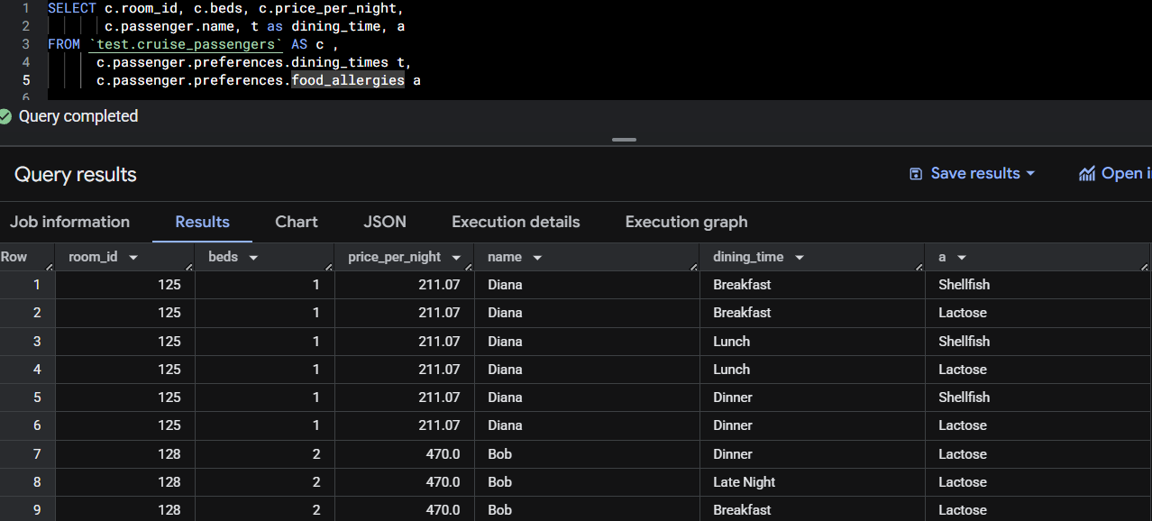
A good way to demonstrate a Cartesian product is through the example below. In the first query, we unnest both dining_times and food_allergies. This causes each combination of those arrays to be returned, which results in duplicated dining_times because BigQuery produces a row for every possible pairing between the two arrays.
In the second query, we unnest only dining_times and leave food_allergies in its original array format. This prevents duplication, and each dining time is listed once per passenger while the full list of food allergies remains nested in its column.
Example 1: unnesting dining_times & food_allergies
Example 2: unnesting dining_times only

How to filter with UNNEST():
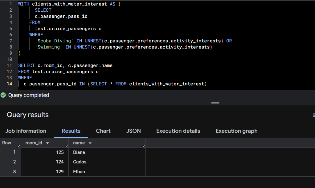
In the example below, we demonstrate how to filter for passengers with water-related interests. When filtering values inside an array, there's no need to perform a cross join, we can simply use UNNEST() within the WHERE clause.
In this example, we first create a CTE that searches for passengers with "Scuba Diving" or "Swimming" listed in their activity_interests. We then pass those matching pass_id values into the main query to retrieve relevant passenger details.
Aggregation with implicit UNNEST():
In the example below, we demonstrate how to perform aggregation on a nested array using implicit UNNEST(). Since onboard_purchases is an array of structs, we first unnest it in the FROM clause, which creates a row for each purchase. This allows us to easily access the cost field for aggregation using dot notation.
The query calculates the total amount spent by each passenger and orders the results by total spend in descending order:
